Can We Optimize the Wagner-Fischer Algorithm?¶

Answer: Yes.

Author:: Fujimoto Seiji
Published:: 2019-07-01
Updated:: 2020-04-26
Copyright:: This document has been placed in the public domain.

1. Introduction¶

In this expository note, I explain several techniques to optimize the Wagner-Fischer algorithm.

This note contains a small benchmark test program as well. The result suggests that it is possible to reduce the computation time by 20-40% in general cases.

2. How to Reduce Memory Usage¶

It is often claimed that the Wagner-Fischer is an \(O(mn)\) space algorithm. Since we need to handle a \((m + 1)(n + 1)\) matrix, it might feel obvious that we need \(O(mn)\) buffer for that computation.

However, there is a rather simple technique to reduce the memory usage to \(O(n)\). Here is the outline:

Prepare an array of length \((m + 1)\).
Fill the array with an increasing series \({0, 1, 2, ..., m}\).
Compute the second row of the matrix, while updating the array incrementally.
Repeat step 3 until you reach the last row.

Obviously the most important step is (3). If we can compute a row of DP matrix with an array of size \(O(n)\). we can just repeat the step up to the last row. So how can we do that? The following explanation should clarify it.

2.1. Step-by-step Explanation¶

Suppose we want to compute the Levenshtein distance between ‘ab’ and ‘cd’. In this case, we need to fill the matrix \(M\) of size 3 x 3 as shown below.

   c d
  . . .   buf := [0, 0, 0]
a . . .
b . . .

Let’s solve this matrix using the buffer.

The first row is the easiest part because we just need to fill the buffer with numbers from \(0\) to \(m\).

    c d   buf[0] := 0
  0 1 2   buf[1] := 1
a . . .   buf[2] := 2
b . . .

Moving to the second row, we know that the value of the leftmost cell is 1. But the assignment should be done with care, because \(M_{00}\) is required to compute the next cell \(M_{11}\).

So first we save buf[0] to a temporary variable and then update buf[0]:

    c d
  0 1 2   tmp := buf[0]
a 1 . .   buf[0] := 1
b . . .

Now we can compute \(M_{11}\) using the following values.

buf[0] = the cell to the left
buf[1] = the cell above
tmp    = the cell in the upper left

In other words:

buf[1] = min(buf[0], buf[1], tmp) + 1

To avoid losing information required to compute \(M_{12}\), we need to update the buffer in the following steps.

    c d
  0 1 2   val := min(buf[0], buf[1], tmp) + 1
a 1 1 .   tmp := buf[1]
b . . .   buf[1] := val

In much the same way, we can compute the last cell of the row.

    c d
  0 1 2   val := min(buf[1], buf[2], tmp) + 1
a 1 1 2   tmp := buf[2]
b . . .   buf[2] := val

We can just repeat the procedure to fill the third row. This leads us to the following result.

    c d
  0 1 2   buf = [2,2,2]
a 1 1 2
b 2 2 2

So the distance between ‘ab’ and ‘cd’ turns out to be 2.

2.2. Implementation in Python¶

The following is the straight-forward implementation in Python.

def wagner_fischer_O1(s, t):
    n = len(s)
    m = len(t)
    buf = list(range(m + 1))

    for i in range(1, n + 1):
        tmp = buf[0]
        buf[0] = i

        for j in range(1, m + 1):
            if s[i - 1] == t[j - 1]:
                tmp, buf[j] = buf[j], tmp
            else:
                val = min(buf[j], buf[j - 1], tmp) + 1
                tmp, buf[j] = buf[j], val
  return buf[m]

An interesting aspect of this technique is that it often improves not only the memory usage, but also the computation time as well (only a few percent improvement at best, though).

See the benchmark result below for more details.

3. How to Reduce Computation Time¶

This section explains “generalized” Ukkonen’s optimization.

Ukkonen’s technique is well known; It states that if we don’t mind editing steps that cost more than \(k\), we only need to compute \(n (2k + 1)\) cells at most. [Ukkonen1985]

The less known fact is that we can apply this technique to general cases where there is no threshold parameter.

3.1. Upper Bound Theorem¶

First let me introduce a theorem. Suppose we have two strings \(S\) and \(T\), whose lengths are \(n\) and \(m\) respectively with \(n < m\). We can guarantee that the Levenshtein distance cannot exceed \(m\):

LevenshteinDistance(S, T) < m

Here is a proof. Let’s notate “i-th character of a string X” by \(x_i\). Using this notation, we can write \(S\) and \(T\) as follows.

\[ \begin{align}\begin{aligned}S = s_1 s_2 s_3 ... s_{n-1} s_n\\T = t_1 t_2 t_3 ... t_{m-1} t_m\end{aligned}\end{align} \]

Since \(n < m\), we can rewrite \(T\) to:

\[T = t_1 t_2 t_3 ... t_{n-1} t_n ... t_m\]

Now we can see that we can convert T to S using the following steps.

Substitute the sequence of \(t_1 ... t_n\) to \(s_1 ... s_n\).
Delete \(t_{n+1} ... t_m\).

The cost of performing this operation is at most m (because it needs \(n\) substitutions and \(m - n\) deletions). Thus the theorem has been proved \(\square\)

3.2. Optimization¶

Let’s use this theorem to optimize the algorithm. For starters, let’s focus on the cell in the upper-right corner of a matrix.

For example, if S=’abcd’ and T=’pqrs’, this cell can be shown as below.

    p q r s
  . . . . *
a . . . . .
b . . . . .
c . . . . .
d . . . . .

The thing worth noting here is that there is exactly a single path that goes through the cell i.e. an edit path of \(n\) deletions + \(m\) insertions.

Here is how the path looks like.

    p q r s
  0 1 2 3 4
a . . . . 5
b . . . . 6
c . . . . 7
d . . . . 8

This is indeed the most expensive way to convert \(S\) to \(T\). Since it needs \(n + m\) steps, the cost to follow the path is always \(n + m\).

We know that the edit distance between \(S\) and \(T\) cannot exceed \(m\). So there is no reason to consider a path that costs \(n + m\). This means that the corner cell is irrelevant when computing the edit distance. We can always skip the cell and the final result is still correct.

The same argument can be applied to the other cells as well. For example, let’s consider the cells adjacent to the corner cell.

    p q r s
  . . . *
a . . . . *
b . . . . .
c . . . . .
d . . . . .

Although there are several edit paths that step through either or both of them, such paths always contain the following steps.

\(n - 1\) insertions + \(m - 1\) deletions

Following the reasoning above, if the inequality condition \(m < (m - 1) + (n - 1)\) holds, we can safely ignore these cells. By simplifying the inequality condition, we get \(2 < n\). In other words, unless the length of \(S\) is less than \(2\), we do not need to bother computing these cells.

Let’s generalize this observation. Choose a cell \(C\) in a matrix and denote the Manhattan distance from it to the nearest corner cell (the upper-right one or the lower-left one) by \(D_c\).

Since any path passing through the cell requires \(n - D_c\) insertions + \(m - D_c\) deletions, we can ignore this cell if the condition \(m < (n - D_c) + (m - D_c)\) holds.

In short, we can safely ignore the cells satisfying \(2D_c < n\), and the answer is still correct.

3.3. Actual Example¶

Back to the example above where S = “abcd” and T = “pqrs”. In this case \(m = 4\), thus the following 12 cells satisfy \(D_c < m\).

    p q r s
  . . * * *
a . . . * *
b * . . . *
c * * . . .
d * * * . .

So we need to fill the remaining 13 cells to compute the distance, For example, to fill the cell marked Z below, we only need to consider the cell to the left (marked X) and the cell in the upper- left (marked Y).

    p q r s
  . Y * * *
a . X Z * *
b * . . . *
c * * . . .
d * * * . .

Below shows the matrix after flood-filing. You can see that the edit distance between “abcd” and “pqrs” is computed correctly.

    p q r s
  0 1 * * *
a 1 1 2 * *
b * 2 2 3 *
c * * 3 3 4
d * * * 4 4

3.4. How Can We Implement This?¶

If you are looking for an example implementation, please refer to wagner_fischer_O2() contained in the benchmark script.

4. Benchmark¶

4.1. Method¶

I implemented the three versions of the Wagner-Fischer algorithm.

Wagner-FIscher (no optimization)
Wagner-FIscher + Memory Reduction
Wagner-Fischer + Memory Reduction + CPU Time Reduction

See the benchmark script benchmark.c for details.

4.2. Result¶

The following numbers are retrieved using Intel Core i3-4010U (1.70GHz) with GCC 6.3.0.

Function	TIME[s]	SPEED[calls/s]
wagner_fischer	6.382	657245
wagner_fischer_O1	5.903	710527
wagner_fischer_O2	3.993	1050380

The following graph shows the result graphically.

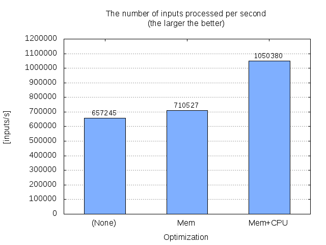
../_images/benchmark2.png — Comparison of the three implementaions of the Wagner-Fischer algorithm.¶